


Summary
Modeling and simulation are key for the iterative development of thermal protection systems (TPS’s) for hypersonic weapons. In this work, the temperature-dependent flexural strength (FS) of α-SiC ceramic is predicted given Young’s modulus, Poisson’s ratio, and temperature. An artificial neural network (ANN) surrogate model is created to retain property-performance prediction while increasing computation speed. The ANN computes many times faster (less than a second vs. tens of minutes) than a finite-element model (FEM). An uncertainty quantification (UQ) is necessary because property inputs vary due to defects in manufacturing processes. Here, the ANN surrogate model provides the necessary computational speedup to perform a UQ. A temperature-dependent UQ is demonstrated using the ANN. This work demonstrates that a machine-learning surrogate model is a useful replacement for a physics-based FEM for predicting the temperature-dependent FS of a TPS with UQ.
Introduction
The United States is currently developing hypersonic weapons [1]. Other countries have been ahead in deploying hypersonic weapons since 2016 [2]. A limiting factor in deploying hypersonics is their TPS’s [3]. Hypersonic flight increases the heat resilience necessary of the weapons’ TPS’s. Without a TPS, critical components of the weapon will likely melt. To engineer a TPS for a hypersonic weapon, physics-based modeling is useful; however, it is slow. Furthermore, due to manufacturing defects, material properties are uncertain and must be considered, placing them outside the computational reach of physics-based simulations. UQ requires many samples of a model to effectively map the uncertainty in material properties to uncertainty in the TPS material’s performance. Here, a fast surrogate model is a substitute for the full physics-based model. This model consists of an ANN with property inputs of Young’s modulus and Poisson’s ratio to FS, a performance measure, as the output.
The most prevalent UQ model of α-SiC is from the 1990s and uses purely data-driven parameters [4]. This model lacks physics, can potentially lead to unrealistic conclusions, and is a fitted logistic function. Silicon carbide is a temperature-resistant lightweight material that is used in hypersonic weapon TPS’s. UQ can coordinate with decision makers in a manufacturing supply chain, where the risk of a material’s failure on its final deployed state is a critical factor influencing decisions [5, 6]. A known problem with ceramics manufacturing is variations in microstructure [7] and surface defects [8, 9] from manufacturing processes. Hypersonic weapons are also exposed to particulates and acoustic waves during flight [10]. Therefore, a need for UQ in ceramics manufacturing is undeniable [11–13]. Recently, an experimentally driven approach has been taken in UQ of FS [14]; however, more developments in a generalizable model would be greatly beneficial.
The computationally light replacement model for the physics-based model is a surrogate model. Surrogate models stand in for the physics-based model and retain the nonlinear mapping from inputs to outputs. The surrogate model always works in tandem with the physics-based model by training on it. The physics-based model is solved with high-performance computing (HPC) and provides quality training data to the surrogate model. While successful in making predictions, physics-based models are computationally expensive [15, 16]. This computational expense limits their usefulness in UQ studies [17]. Even models that compute rapidly with HPC [18] do not approach the speed needed for a surrogate model for UQ. Should quantum computing become ubiquitous, large systems of linear equations that are the kernel of physics-based simulation could provide a powerful solution, but that is a distant horizon [19, 20]. Using the surrogate model here, the uncertainty in Young’s modulus and Poisson’s ratio may be adjusted and the model provides near-instant feedback on the resulting changes in FS uncertainty. The key to this rapid UQ will be the machine-learning (ML) model.
The ML model applied in the ANN converts an input vector, including material properties and temperature, to FS at a wide range of temperatures. In the next section, the ANN theory is summarized and discussed. The implementation of ANN with the backpropagation algorithm is outlined in the ANN Implementation section, where two optimization algorithms are compared. In the ANN Training section, the accuracy of the ANN is tested by randomly removing data from the training set and predicting on those removed data. The number of data records removed is incrementally increased to the breakdown’s limit. A temperature-dependent forward UQ from Young’s modulus and Poisson’s ratio to FS is then conducted using the ANN surrogate model. The interpolation among temperatures not computed by the thermomechanical fracture model is shown to operate properly. The temperature dependence is important for demonstrating the model’s capabilities for hypersonic weapons’ TPS’s. Finally, the outlook for these weapons’ ANN and manufacturing is discussed in the Conclusions section.
ANN Theory
An ANN consists of layers of neurons with connections between them. A neuron stores a value and receives and sends signals (which are essentially values) or numbers. The connections map the output signals from one layer of neurons to the next layer of neurons, where the signals become inputs. Weights on each connection are trained. Each neuron also has a constant bias that is trained. The ANN in this work is supervised by FSs as the labels. The ANN in FS modeling is broken down next.
The general equation for the value of given input χj to a given neuron is
 , , |
(1) |
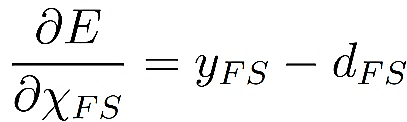
where yi are inputs from neurons from a previous layer and χ j is the sum of the signals to neuron index j closer to the outputs [21]. wji proceeds from left neuron index i nearer to inputs to right neuron j nearer to outputs. A bias for a given neuron is added with an additional input value of 1, and its weight is then treated the same as other weights. Next, the cost function, or error E, is defined with the difference of the lab’eled data point and the output from the ANN as
| (2) |
where dFS is the labeled data point and yFS is the output from the ANN, given the inputs and weight values [21]. To minimize the cost function, E, the gradient or sensitivity of the cost E to each of the weights is sought. The naive way to obtain the gradient would be to perturb each weight one at a time by reevaluating the ANN at every step. Obtaining the gradient would be a computationally expensive process. Backpropagation is a computationally efficient algorithm to provide the gradient.
In the backpropagation algorithm, the ANN is only run forward one time. All the χ’s and y’s are found from the forward pass. Expressions for the gradient are written using derivatives and the chain rule from calculus. These expressions are orders of magnitude less computationally burdensome than evaluating the entire ANN again. Starting with the output layer, the partial derivative is taken for the output signal, yFS, as follows [21]:
 , , |
(3) |
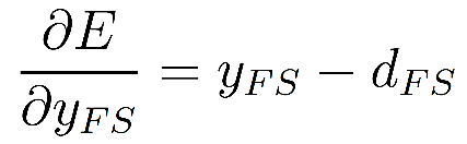
The derivative of the cost regarding the total of the input signals to the output neuron yFS is taken as
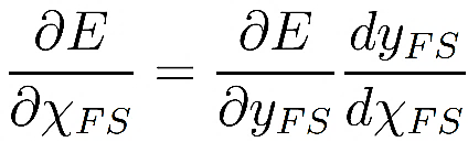 , , |
(4) |
The term ∂E/∂yFS is known from equation 3. χFS is the total input to the neurons in the final layer. The term dyFS/dχFS is the derivative of the output signal for the total inputs. The rectified linear unit activation function is used in this work to prevent obtaining negative output [22]. The rectified linear unit activation is as follows [21]:
| (5) |
For numbers greater than 0, dyFS/dχFS = 1. Thus, equation 4 becomes
 , , |
(6) |
From here, the gradient regarding the weights is needed. The derivative is written for the cost function for weights wFSi on the signals leading to the final layer as follows [21]:
| (7) |
The expression ∂E/∂χFS is known from equation 6. The expression ∂χFS/∂wFSi equals yi, the signals from the last layer before the output layer (see equation 1). The process backpropagates to obtain the gradient for all the weights. Figure 1 shows the last layer of the neural network where the backpropagation algorithm begins. Figure 2 displays the input parameters and output prediction of the neural network, which has two layers between inputs and outputs and is 50 or 100 neurons wide.
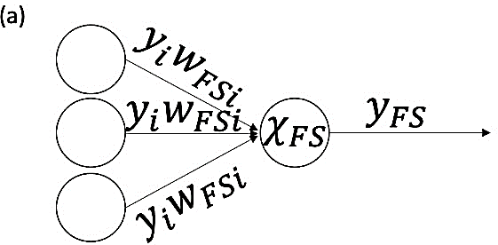
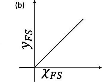
Figure 1. ANN Near the FS Output: (a) End of Neural Network and (b) Rectified Linear Unit Signal (Source: E. Walker, J. Sun, and J. Chen).
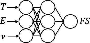
Figure 2. Inputs and Outputs of the ANN Surrogate Model (Source: E. Walker, J. Sun, and J. Chen).
ANN Implementation
Key computational details about ANN include the number of hidden layers between inputs and outputs, the width or number of neurons in those hidden layers, the activation function, and the algorithm choice for optimizing weights during training. The ANN in this work uses widths of hidden layers of about 100 neurons. After several tests, two hidden layers are deemed necessary and used. Dropping to one hidden layer decreases the R2 on fitting back to the training data to 0.994. A near-perfect R2 of 1 is expected in this scenario of predicting the same data used for training. Adding a second hidden layer does not increase the computation time by a noticeable amount. The weights are trained by a (limited memory) Broyden-Fletcher-Goldfarb-Shanno (BFGS) [23] algorithm. The maximum number of iterations to optimize the weights is set to 500. Poisson’s ratio is on a smaller scale than Young’s modulus and temperature. The inputs are rescaled to improve the training performance.
BFGS is a quasi-Newton method to minimize the cost function. It includes curvature information via a Hessian matrix in its search. The Hessian contains second derivatives of the cost function regarding the weights. A starting point for BFGS is Newton’s method [23]:
| (8) |
where k is the iteration index, x is the vector of weights, and H is the Hessian. The inverse of the Hessian matrix is taken in Newton’s method. However, since matrix inversion is computationally expensive, an approximation to the inverse Hessian matrix [H]−1 is computed instead. The gradient supplied by backpropagation is gk. A scalar number α controls step size and is optimized at each iteration in BFGS. The BFGS updated equations are listed next. For x0 in the initial guess state, a starting approximation matrix of the inverse Jacobian, H0, is guessed. A new compact variable s is defined by the following [23]:
| (9) |
Then, the cost function E from equation 2 is minimized by introducing a scalar αk,
 , , |
(10) |
where xk is the current vector of weights and biases. sk is set by equation 9. Therefore, in equation 10, the only variability in the cost function E(αk) is due to αk. Methods exist to minimize E(αk) by changing αk [23]. Next, another compacted variable σ is introduced as
| (11) |
The weights and biases are updated as
| (12) |
The approximate inverse Hessian matrix is updated as
| (13) |
where the key update matrix D is obtained by satisfying another equation:
| (14) |
where y is another compacted variable from other known variables,
| (15) |
Another solver is a stochastic gradient-based approach known as “Adam” [24]. Parameters are updated with
 , , |
(16) |
The difference thus far from BFGS is that the Hessian matrix is not used in the update but rather parameters that are functions of g, m̂, and v̂, with ϵ as a constant hyperparameter. Adam is suited for large amounts of noisy training data [24]. As a test, BFGS and Adam were used to train two otherwise identical neural networks. The two trained neural networks were predicted back on the training data. BFGS was more accurate than Adam, as measured by R2.
The ANN after training by BFGS will be run many times to predict FS, the output of choice in this study. This forward UQ maps the uncertainty in the three inputs to the FS. The inputs are sampled according to their probability density functions (pdf’s).
ANN Training
The training data set used in this study comes from a three-way coupled thermomechanical fracture model solved by the FEM. There are extensive efforts of developing physics-based simulations which can be used to study the bending, buckling, vibration, and stress intensity of various shapes of materials [18, 25–28]. Various attempts have been made to model the fracture behavior of brittle materials like ceramics [29–32]. The model generates the training data set on the FS of α-SiC over a wide range of temperatures, which is particularly helpful for applications like thermoprotection systems [33]. The three-way coupling model consists of modules, including elastic mechanics, phase field for damage, and heat conduction. The phase field uses an auxiliary scalar field to model material damage. This field is used to capture both the history of strain energy and the weakening effect on material properties as damage accumulates. The evolution of damage is governed by the Allen-Cahn equation [29, 30, 32]. The material properties are obtained from experimental data by Munro [4]. The simulation setup is based on a standard four-point bending test specified in ASTM C1161-18 [34]. The point of fracture is determined according to the Griffith theory [35]. The cell size is controlled to be small enough to capture the fracture surface [29, 30]. FS is defined as the maximum tensile stress that the specimen sustains before cracking.
The temperatures of the training data set from the numerical simulation are 400, 600, 800, 1000, 1200, and 1400 °C. The mean Young’s modulus is as follows [4]:
| (17) |
and the mean Poisson’s ratio is
| (18) |
Together with the mean, four combinations of E±3% and ν±25% at each temperature fill out the parameter space as suggested by the experimental data [4]. There are five training points at each of the six temperatures, totaling 30 training points. The five data points are the mean of E and ν, the upper bound of E with the upper bound of ν, the upper bound of E with the lower bound of ν, the lower bound of E with the upper bound of ν, and the lower bound of E with the lower bound of ν. For Young’s modulus and Poisson’s ratio, respectively, 3% and 25% are taken as the three standard deviations distance or 99% confidence interval when performing the forward UQ later. Each training data point consists of the three input parameters—Young’s modulus, a Poisson’s ratio, and a temperature, resulting in FS as the output. A similar approach was taken by Nagaraju et al. [36]. However, this work used an ANN and included adding temperature variation, 400–1400 °C, to emphasize the temperature effect.
After the ANN is trained by the 30 data points, a rigorous cross-validation test of the ANN accuracy is conducted and summarized in Figure 3 [37], where the FEM [33] provides 30 FS’s from inputs to complete the training data set. Of the data set of 30 points, n data are selected randomly to move from training to testing. For instance, when n = 3, the training data set size is 27 and the testing data set size is 3. The ANN, after being trained on 27 data, predicts on 3 data. The R2 tends to decrease with shrinking training data set size because less and less of the parameter space is covered during training. In Figure 4, five trials are conducted at each n. When n = 7, the first negative R2 appeared. Therefore, the ANN is reliable with an n smaller than 7.
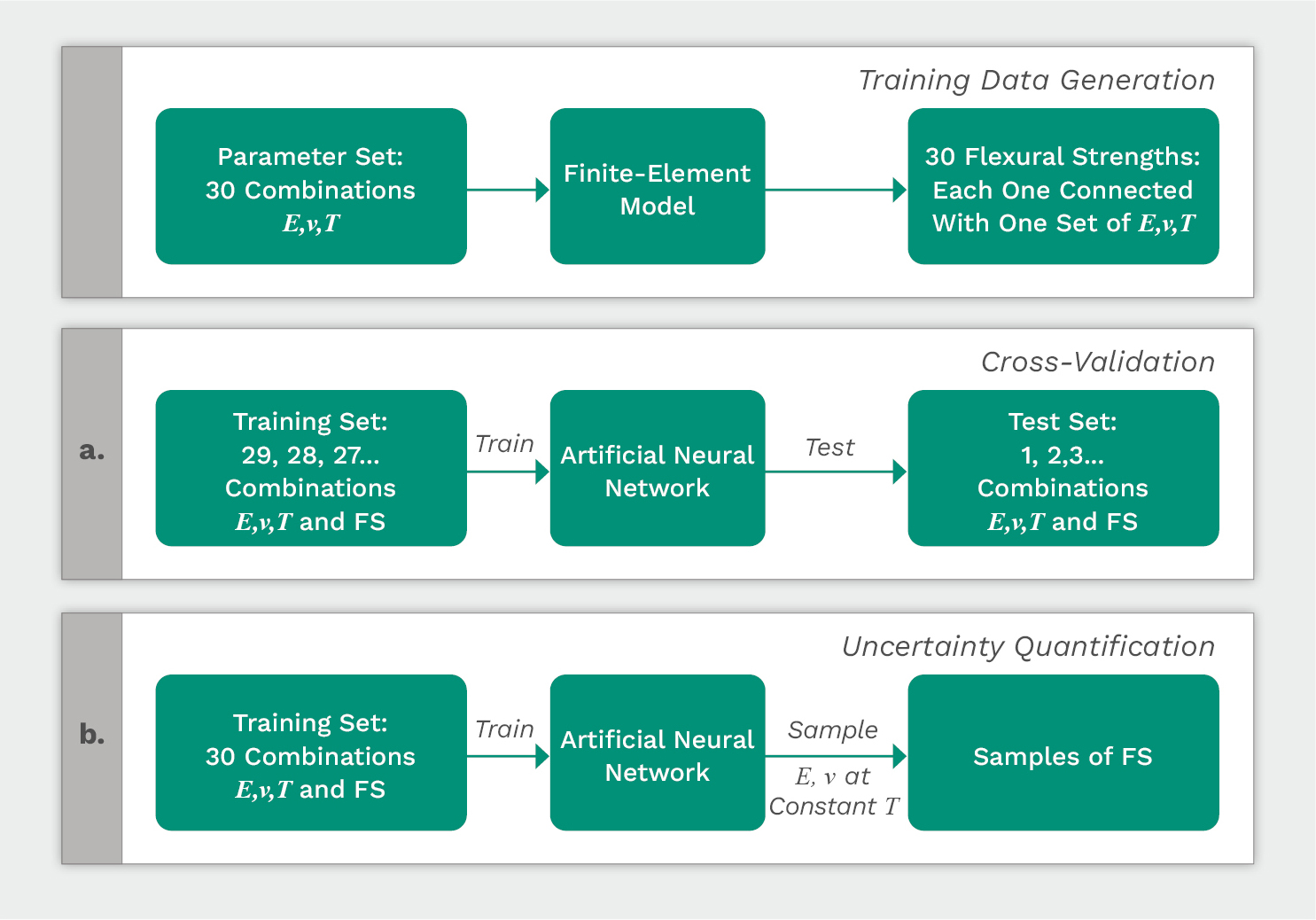
Figure 3. The FEM Training Data Set: (a) Cross-Validation for the ANN Reliability and (b) Forward UQ (Source: E. Walker, J. Sun, and J. Chen).
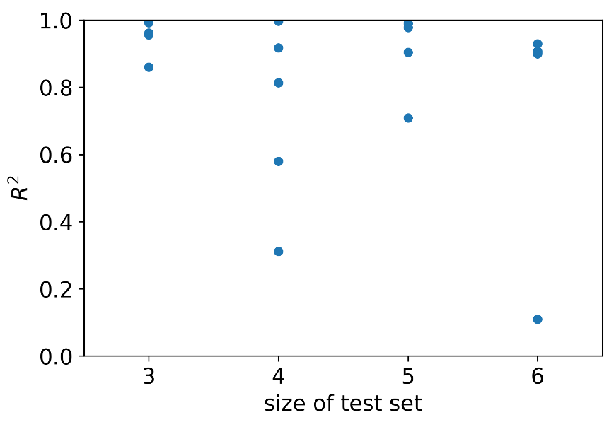
Figure 4. Cross-Validation of the ANN (Source: E. Walker, J. Sun, and J. Chen).
The process employed for validating the ANN is known as cross-validation [37]. The loss in reliability may be attributed to declining dimensionality of the training data or the variety in Young’s modulus, Poisson’s ratio, and temperature.
Now that the ANN is trained, one million samples are used for a forward UQ of α-SiC at 1400 °C (Figure 5) as an example. Both Young’s modulus and Poisson’s ratio are modeled as Gaussian. Their mean and standard deviation are also displayed in Table 1. For future studies, a Bayesian update could be used to change the means and standard deviations of Young’s modulus and Poisson’s ratio as more experimental data become available [38].
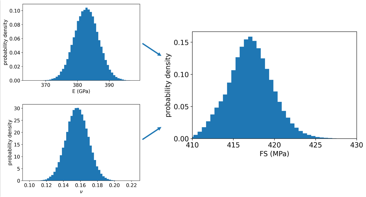
Figure 5. A Forward UQ for FS at 1400 °C (Source: E. Walker, J. Sun, and J. Chen).
Table 1. Uncertainty Shape Parameters of the Gaussian Distributions
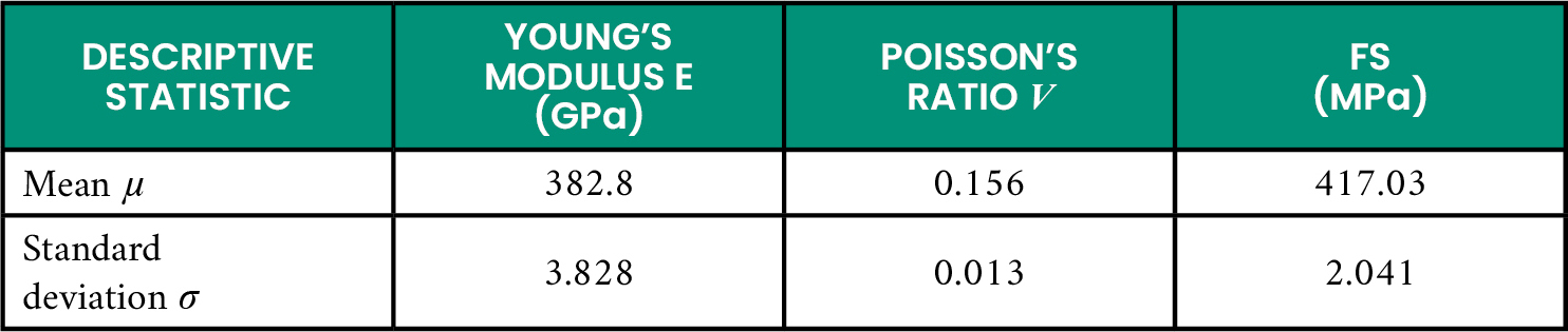
Figure 5 shows the UQ of FS of α-SiC at 1400 °C as an example. The mean of predicted FS is 417.03 MPa, compared with 416.84 MPa computed by the physics-based model. The ANN therefore achieves consistency with the physics-based model. With this tool, a manufacturer can rely on the ANN framework to predict the mechanical strength of α-SiC within seconds during each design iteration. The uncertainty has also been quantified at a standard deviation of 2.041 MPa. The entire training data set was used for the UQ conducted here. More training data will help stabilize the surrogate model.
The ANN is effective at capturing FS given its nonlinear dependence on temperature. Figure 6 displays the mean FS of the ANN as a function of temperature, labeled as circles, and its 95% confidence interval. The thermomechanical fracture model solved via FEM, serving as the benchmark data, is overlaid with x’s. The 95% confidence interval of the ANN is ±2σ from the mean. The uncertainty of the ANN is temperature dependent—at its maximum, σ = 2.36 (MPa) at 800 °C; at its minimum, σ = 1.36 (MPa) at 1200 °C.
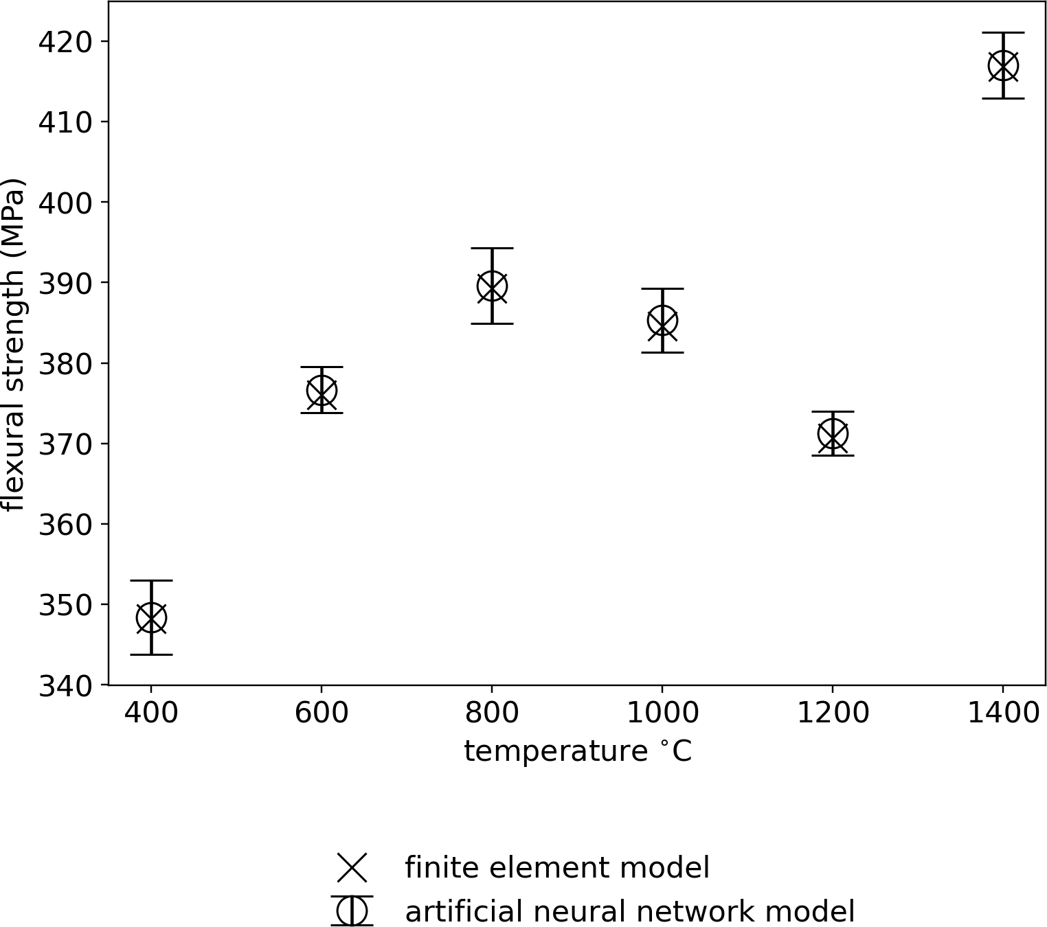
Figure 6. NANN and Physics Model Solved With FEM Prediction of FS vs. Temperature (Source: E. Walker, J. Sun, and J. Chen).
All distributions for the inputs in Table 1, namely Young’s modulus and Poisson’s ratio, are assumed as Gaussian and functions of temperature (equations 17 and 18). When defining the pdf of Young’s modulus, three standard deviations are set to 25% of the mean. The same procedure is taken for defining the pdf of Poisson’s ratio except for using 3% of the mean. To validate the smooth interpolation between training data temperatures, predictions are made and plotted in Figure 7.
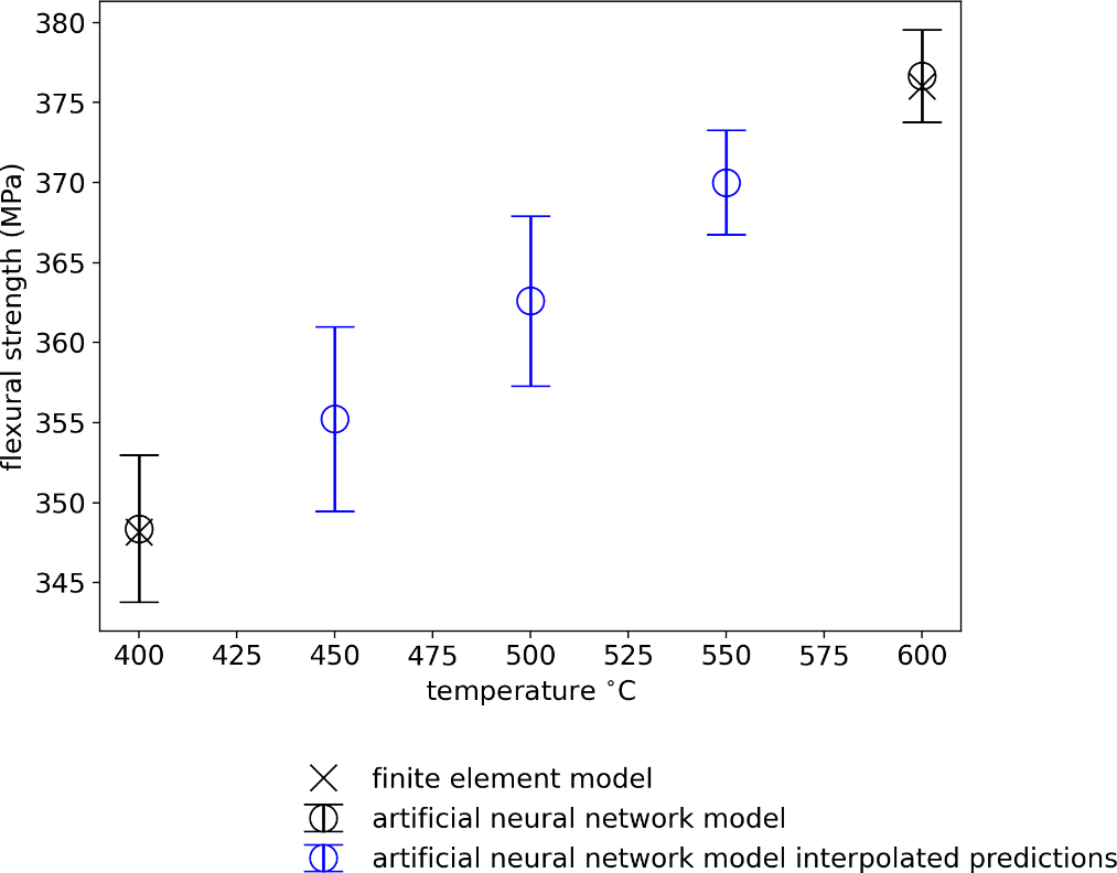
Figure 7. Interpolation Prediction of FS vs. Temperature (Source: E. Walker, J. Sun, and J. Chen).
The choice of three standard deviations in this work contrasts against absolute bounds because the Gaussian distribution used here has no absolute bounds. Munro [4] has the uncertainty at ±25% for Young’s modulus and ±3% for Poisson’s ratio as absolute uncertainty bounds. However, a Gaussian distribution has infinitely long bounds. It should be noted that 99.5% of the samples are within ±3σ of the mean for a Gaussian pdf. Therefore, the choice of three standard deviations depends mostly on the literature precedent of uncertainties in α-SiC properties. The samples of the inputs are passed through the ANN, with FS samples as the output. The mean and standard deviation of the FS samples are taken at each temperature. The temperature reliance is from the oxidation of the surface [39] that increases FS.
Conclusions
The surrogate model shown here will prove useful for designing TPS’s of hypersonic weapons. If manufacturing defects persist, there will be a need for UQ; this is enabled through the surrogate model. The surrogate model in this work is an ANN, and it has been cross-validated for accuracy. The results from the ANN cross-validation show that the training data set must contain enough of the nonlinear behavior of FS to exhibit reliable accuracy. The presented ANN is also used in an effective temperature-dependent UQ demonstration as a surrogate model. The reliability and accuracy of ANNs should remain in the parameter space of the training data. This study arrives at a similar conclusion. Rodríguez-Sánchez [40] used an ANN to model low-velocity impact force in a thermoplastic elastomer material (the ANN is accurate to 1% within the region of the training data).
Without UQ, designers of hypersonic weapons have no hint of the risk of their TPS’s lacking FS during flight. The computation time of the presented work is greatly improved from the physics-based simulation. The parallelized physics-based simulation running on a cluster requires tens of minutes to complete a case. Run on a single processor, the ANN only requires seconds to train. An ANN prediction after training is faster—less than a second. Prediction of one million parameter samples requires seconds to run. With the modeling advancement shown here, the iterative step has been made in designing hypersonic weapons.
Questions regarding the future of ML in thermal protection systems modeling depend on how much physics is modeled by the ANN. For a separate application, As’ad et al. used physics-based constraints on an ANN to model stress and strain of elastic materials [41]. Those constraints include dynamic stability, objectivity, and consistency.
Acknowledgments
Funding for this project was provided, in part, by LIFT, the Detroit-based national manufacturing innovation institute operated by the American Lightweight Materials Manufacturing Innovation Institute, a Michigan-based nonprofit, 501(c)3 as part of ONR Grant N00014-21-1-2660.The authors are grateful to Dr. Amberlee Haselhuhn and Dr. David Hicks for the constructive discussions.
References
- Sayler, K. M. “Hypersonic Weapons: Background and Issues for Congress.” Congressional Research Service, 2023.
- Fleeman, E. “A Historical Overview of a Half Century of U.S. Missile Development.” DSIAC Journal, vol. 3, no. 3, 2016.
- Lietha, M. N., and D. T. Motes III. “Understanding Thermal Protection Systems and the Development of the Hypersonic Speed Regime in the United States.” Defense Systems Information Analysis Center (DSIAC) State-of-the-Art Report, DSIAC-2020-1326, December 2020.
- Munro, R. G. “Material Properties of a Sintered alpha-SiC.” Journal of Physical and Chemical Reference Data, vol. 26, pp. 1195–1203, 1997.
- Alemany, M. M. E., F. Alarcón, F.-C. Lario, and J. J. Boj. “An Application to Support the Temporal and Spatial Distributed Decision-Making Process in Supply Chain Collaborative Planning.” Computers in Industry, vol. 62, pp. 519–540, 2011.
- Souifi, A., Z. C. Boulanger, M. Zolghadri, M. Barkallah, and M. Haddar. “Uncertainty of Key Performance Indicators for Industry 4.0: A Methodology Based on the Theory of Belief Functions.” Computers in Industry, vol. 140, 2022.
- Fan, H., W. T. Ang, and X. Wang. “On the Effective Property of a Micro-Cracked and a Microscopically Curved Interface Between Dissimilar Materials.” Forces in Mechanics, vol. 7, 2022.
- Boljanović, S., and A. Carpinteri. “Modelling of the Fatigue Strength Degradation Due to a Semi-Elliptical Flaw.” Forces in Mechanics, vol. 4, 2021.
- Dong, G., C. Lang, C. Li, and L. Zhang. “Formation Mechanism and Modelling of Exit Edge-Chipping During Ultrasonic Vibration Grinding of Deep-Small Holes of Microcrystalline-Mica Ceramics.” Ceramics International, vol. 46, no. 8, part B, pp. 12458–12469, 2020.
- Knight, T. “Small Particle Effects on Hypersonic and Subsonic Flight Vehicles.” DSIAC Technical Inquiry Response Report, DSIAC-BCO-2021-178, May 2021.
- Behnam, A., T. J. Truster, R. Tipireddy, M. C. Messner, and V. Gupta. “Uncertainty Quantification Framework for Predicting Material Response with Large Number of Parameters: Application to Creep Prediction in Ferritic-Martensitic Steels Using Combined Crystal Plasticity and Grain Boundary Models.” Integrating Materials and Manufacturing Innovation, vol. 11, pp. 516–531, 2022.
- Saunders, R., A. Rawlings, A. Birnbaum, A. Iliopoulos, J. Michopoulos, D. Lagoudas, et al. “Additive Manufacturing Melt Pool Prediction and Classification via Multifidelity Gaussian Process Surrogates.” Integrating Materials and Manufacturing Innovation, vol. 11, pp. 497–515, 2022.
- Nitta, K. H., and C. Y. Li. “A Stochastic Equation for Predicting Tensile Fractures in Ductile Polymer Solids.” Physica A: Statistical Mechanics and its Applications, vol. 490, pp. 1076–1086, 2018.
- Štubňa, I., P. Šín, A. Trník, and L. Vozár. “Measuring the Flexural Strength of Ceramics at Elevated Temperatures – An Uncertainty Analysis.” Measurement Science Review, vol. 14, pp. 35–40, 2014.
- Panchal, J. H., S. R. Kalidindi, and D. L. McDowell. “Key Computational Modeling Issues in Integrated Computational Materials Engineering.” Computer-Aided Design, vol. 45, pp. 4–25, 2013.
- Shi, J., T. Cook, and J. Matlik. “Integrated Computational Materials Engineering for Ceramic Matrix Composite Development.” The 53rd AIAA/ASME/ASCE/AHS/ASC Structures, Structural Dynamics and Materials Conference, 2012.
- Sepe, R., A. Greco, A. D. Luca, F. Caputo, and F. Berto. “Influence of Thermo-Mechanical Material Properties on the Structural Response of a Welded Butt-Joint by FEM Simulation and Experimental Tests.” Forces in Mechanics, vol. 4, 2021.
- Yaylaci, M. “Simulate of Edge and an Internal Crack Problem and Estimation of Stress Intensity Factor Through Finite Element Method.” Advanced Nano Research, vol. 12, pp. 405–414, 2022.
- Becerra, A., A. Prabhu, M. S. Rongali, S. C. S. Velpur, B. Debusschere, and E. A. Walker. “How a Quantum Computer Could Quantify Uncertainty in Microkinetic Models.” The Journal of Physical Chemistry Letters, vol. 12, no. 29, pp. 6955–6960, 2021.
- Becerra, A., O. H. Diaz-Ibarra, K. Kim, B. Debusschere, and E. A. Walker. “How a Quantum Computer Could Accurately Solve a Hydrogen-Air Combustion Model.” Digital Discovery, vol. 1, pp. 511–518, 2022.
- Rumelhart, D. E., G. E. Hinton, and R. J. Williams. “Learning Representations by Back-Propagating Errors.” Nature, vol. 323, pp. 533–536, 1986.
- Nair, V., and G. Hinton. “Rectified Linear Units Improve Restricted Boltzmann Machines.” Proceedings of the 27th International Conference on Machine Learning, pp. 807–814, June 2010.
- Shanno, D. F. “Conditioning of Quasi-Newton Methods for Function Minimization.” Mathematics of Computation, vol. 24, 1970.
- Kingma, D. P., and J. Ba. “Adam: A Method for Stochastic Optimization.” International Conference on Learning Representations, 2015.
- Van Vinh, P., N. Van Chinh, and A. Tounsi. “Static Bending and Buckling Analysis of Bi-Directional Functionally Graded Porous Plates Using an Improved First-Order Shear Deformation Theory and FEM.” European Journal of Mechanics – A/Solids, vol. 96, 2022.
- Cuong-Le, T., K. D. Nguyen, H. Le-Minh, P. Phan-Vu, P. Nguyen-Trong, and A. Tounsi. “Non-Linear Bending Analysis of Porous Sigmoid FGM Nanoplate via IGA and Nonlocal Strain Gradient Theory.” Advances in Nano Research, vol. 12, pp. 441–455, 2022.
- Kuma, Y., A. Gupta, and A. Tounsi. “Size-Dependent Vibration Response of Porous Graded Nanostructure With FEM and Nonlocal Continuum Model.” Advances in Nano Research, vol. 11, pp. 1–17, 2021.
- Alimirzaei, S., M. Mohammadimehr, and A. Tounsi. “Nonlinear Analysis of Viscoelastic Micro-Composite Beam With Geometrical Imperfection Using FEM: MSGT Electromagnetoelastic Bending, Buckling and Vibration Solutions.” Structural Engineering and Mechanics, vol. 71, pp. 485–502, 2019.
- Miehe, C., F. Welschinger, and M. Hofacker. “Thermodynamically Consistent Phase-Field Models of Fracture: Variational Principles and Multi-Field FE Implementations.” International Journal for Numerical Methods in Engineering, vol. 83, pp. 1273–1311, 2010.
- Miehe, C., L. Schänzel, and H. Ulmer. “Phase Field Modeling of Fracture in Multi-Physics Problems. Part I. Balance of Crack Surface and Failure Criteria for Brittle Crack Propagation in Thermo-Elastic Solids.” Computer Methods in Applied Mechanics and Engineering, vol. 294, pp. 449–485, 2015.
- Zhang, X., C. Vignes, S. W. Sloan, and D. Sheng. “Numerical Evaluation of the Phase-Field Model for Brittle Fracture with Emphasis on the Length Scale.” Computational Mechanics, vol. 59, pp. 737–752, 2017.
- Clayton, J. D., R. B. Leavy, and J. Knap. “Phase Field Modeling of Heterogeneous Microcrystalline Ceramics.” International Journal of Solids and Structures, vol. 166, pp. 183–196, 2019.
- Sun, J., Y. Chen, J. J. Marziale, E. A. Walker, D. Salac, and J. Chen. “Damage Prediction of Sintered alpha-SiC Using Thermo-mechanical Coupled Fracture Model.” Journal of the American Ceramic Society, accepted for publication, 2022.
- American Society for Testing and Materials (ASTM) C1161-18. “Standard Test Method for Flexural Strength of Advanced Ceramics at Ambient Temperature,” 24 February 2023.
- Kendall, K. “Chapter 6 – Improving Fracture Mechanics (FM): Let’s Get Back to Energy.” In Crack Control, edited by K. Kendall, editor, Elsevier, pp. 137–163, 2021.
- Nagaraju, H. T., J. Nance, N. H. Kim, B. Sankar, and G. Subhash. “Uncertainty Quantification in Elastic Constants of SiCf/SiCm Tubular Composites Using Global Sensitivity Analysis.” Journal of Composite Materials, vol. 57, pp. 63–78, 2023.
- Walker, E., J. Kammeraad, J. Goetz, M. T. Robo, A. Tewari, and P. M. Zimmerman. “Learning to Predict Reaction Conditions: Relationships Between Solvent, Molecular Structure, and Catalyst.” Journal of Chemical Information and Modeling, vol. 59, pp. 3645–3654, 2019.
- Walker, E. A., K. Ravisankar, and A. Savara. “CheKiPEUQ Intro 2: Harnessing Uncertainties From Data Sets, Bayesian Design of Experiments in Chemical Kinetics.” ChemCatChem, vol. 12, no. 21, pp. 5401–5410, 2020.
- Arai, Y., R. Inoue, K. Goto, and Y. Kogo. “Carbon Fiber Reinforced Ultra-High Temperature Ceramic Matrix Composites: A Review.” Ceramics International, vol. 45, pp. 14481–14489, 2019.
- Rodríguez-Sánchez, A. E. “An Artificial Neural Networks Approach to Predict Low-Velocity Impact Forces in an Elastomer Material.” Simulation, vol. 96, pp. 551–563, 2020.
- As’ad, F., P. Avery, and C. Farhat. “A Mechanics-Informed Artificial Neural Network Approach in Data-Driven Constitutive Modeling.” International Journal for Numerical Methods in Engineering, vol. 123, pp. 2738–2759, 2022.
Biographies
Eric Alan Walker is a research scientist who applies artificial intelligence to new technologies and scientific challenges. His background is in chemical engineering, with a focus on artificial intelligence and data science. In recent years, he has learned integrated computational materials engineering and manufacturing from his colleagues. Dr. Walker holds a Ph.D. in chemical engineering.
Jason Sun is a third-year Ph.D. candidate majoring in aerospace engineering at the University at Buffalo (UB) under the advisement of Dr. James Chen. His research focuses on computational mechanics, multiscale modeling, and integrated computational materials engineering development for ceramic matrix composites. Mr. Sun holds a B.S. in mechanical and aerospace engineering and a B.A. in mathematics from UB.
James M. Chen is an associate professor in the Department of Mechanical and Aerospace Engineering at UB. He has published ~50 peer-reviewed journal articles in multiscale computational mechanics, theoretical and computational fluid dynamics, and atomistic simulation for thermoelectromechanical coupling. His research at the Multiscale Computational Physics Lab has been recognized by numerous media outlets, including a feature article in Aerospace Testing International (UK) and a radio show in Austria. He is a fellow of the American Society of Mechanical Engineers and an associate fellow of the American Institute of Aeronautics and Astronautics. Dr. Chen holds a B.S. in mechanical engineering from National Chung-Hsing University, an M.S. in applied mechanics from National Taiwan University, and a Ph.D. in mechanical and aerospace engineering from The George Washington University.