


Onward with 3D Animations
In Part 1 of this two-part series on blast data visualization article (see the fall 2014 edition of the DSIAC Journal), we learned how to turn simple test data into professional-looking, full-color two-dimensional (2-D) graphs using Python and Matplotlib. However, most people would agree that animations are generally more interesting to watch than a static 2-D illustration. Thus, in Part 2, we now discuss how to use Python and VPython to take test data visualization to the next level by creating (three-dimensional) 3-D animations from blast test data that one might have on hand.
First, let’s examine a few sample data plots produced by a Python program called Test_Data_Animate.py. This application is available at http://www.piezopy.org/ under the code snippets pull-down menu. To operate this program, one will need a text file containing acceleration data from accelerometers mounted to four corners of a test plate exposed to blast loading. As illustrated in Figure 1, the program works by calculating velocity and displacement using composite trapezoidal rule numerical integration, as well as plots acceleration, velocity, and displacement data.

Figure 1: Sample Blast Test Data
Using these data, the program generates a navigable 3-D display window containing a 3-D animation of the motion of the plate, as illustrated in Figure 2. (One can also observe the full-motion video of this animation at http://www.piezopy.org/ under the videos pull-down menu.)
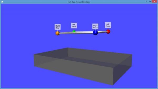
Figure 2: 3‐D Animation of Blast Test Data
Before we dive into a detailed description of the code’s operation, let’s take a step back and consider the physics and math used to create an animation based on these data and what we know about its origins. If one had the opportunity to watch the actual test, one would have seen the plate exposed to the blast physically move in response to the blast loading. Capturing the motion that took place in the physical world and recreating this motion in the virtual (computer-based graphics) world is our goal. So how do we do this? First, we must recognize that the motion of an object is simply a change in its position with respect to time. Change in position is also known as displacement, which is typically measured in our physical space in three dimensions. To create a 3-D animation, one needs to be able to track the physical displacement of an object in all three dimensions and then translate the data into a virtual 3-D coordinate system. So displacement is needed in three dimensions. However, as mentioned previously, our measured test data will only provide the acceleration in the vertical dimension for the four corners of a plate. Fortunately, we can derive what we need from this measured data assuming the following statements are true:
- The plate has a starting position that is parallel with the ground.
- The horizontal and lateral positions of one of the corners remain constant throughout the test.
- The length and width dimensions of the plate do not change.
If all of these conditions are true, then we can leverage these initial conditions and physical constraints to derive the horizontal and lateral displacement of the plate from the relative vertical displacement at the four corners. So how do we get displacement from acceleration? This is where some mathematics comes in. Calculus provides us a convenient method for describing the rate of change of something with respect to something else—for example, the rate of change of displacement with respect to time (velocity) or the rate of change of velocity with respect to time (acceleration). Because acceleration is related to velocity and displacement, with a little calculus we can derive the displacement data we need for our animation from the acceleration data we measured during the blast test. To do this, let’s first refresh our understanding of calculus and how we are going to apply it in this application.
There are two main branches of calculus, differential calculus and integral calculus, and they are inverse operations of each other. Differential calculus will be applied to take us from displacement to velocity and from velocity to acceleration by calculating derivatives. Integral calculus will be applied to take us in the opposite direction by calculating integrals. So in our application, we use integral calculus to go from acceleration to velocity to displacement. More specifically, we use numerical integration, for which we have some readily available Python functions based on validated algorithms. Armed with this information, let’s step through Test_Data_Animate.py a few lines at a time to examine exactly how the Python code can be used to derive velocity and displacement data from acceleration data and how we can generate a 3-D animation from these data.
Our first step is to import the required modules, as indicated in the source code pictured in Figure 3, to extend Python’s capabilities to include scientific computing (numpy), a plotting graphics library (matplotlib), text file reading and writing (csv), numerical integration (scipy.integrate), a 3-D graphics module (visual, aka vpython), and a time clock utility (time).
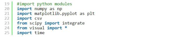
Figure 3: Python Module Import Source Code
The next section of the program contains three separate functions: samplecount(), construct(), and samplerate(), as indicated in the source code pictured in Figure 4. These are subprograms that take in input arguments from the main program and return an output as requested by the main program.
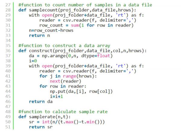
Figure 4: Required Python Functions
The following steps are executed by the main program.
Step 1: Identify the data file and specify the data to be read in from the file.
The source code pictured in Figure 5 is used to accomplish this step. We described file structure of the Plate_Inputs.txt file in Part 1 of this article series.
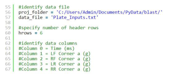
Figure 5: Identify Data File and Data Columns
Step 2: Read the data into separate arrays for each data column.
Before we read the data into arrays, we need to count the number of data rows to be processed. This will provide the length of each data array, which is the number of samples (n) for each measurement type. A call to the samplecount() function, pictured in Figure 6, with the required inputs is used to obtain the result. The samplecount() function uses the csv module to count the total number of rows in the file and then subtracts the number of header rows to get n.

Figure 6: Count Data Samples
Now that we know the number of samples, we are ready to read the data values into five separate arrays: t for the time measurements, and LF_a, RF_a, LR_a, and RR_a for the vertical acceleration measurements. Five separate calls to the construct() function, pictured in Figure 7, are used. The construct() function uses the csv module to read each measurement in a specified column of data and then stores these values in the assigned array.
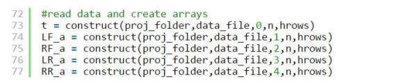
Figure 7: Read Data and Create Arrays
Step 3: Calculate sample rate (sr) and time step (dt).
The sample rate (sr), given in samples/second, is the rate at which data were recorded during the test event. The time step (dt), given in seconds, is the reciprocal of sample rate and is the time interval between samples. Both sr and dt are used in the animation process. To make these calculations more straightforward, we can shift the time array to start at zero and convert the time data units from milliseconds to seconds, as pictured in Figure 8. A call to the samplerate() function on line 86 with the required inputs is used to obtain sample rate. The time step is easily obtained by the calculation on line 89.
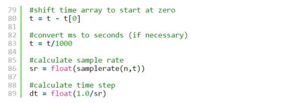
Figure 8: Source Code for Calculating sr and dt
Step 4: Use numerical integration to calculate velocity and displacement.
Numerical methods are used for solving equations or mathematical models too complicated or too time-consuming for an analytic solution. Using integral calculus to obtain velocity and displacement data from our blast response data is a perfect example of this type of problem. There are numerous methods available for numerical integration. We will focus on a method called composite trapezoidal rule numerical integration, which is well-suited to our task.
To refresh everyone’s memory, there are two types of integrals in calculus, definite and indefinite. An indefinite integral is solved for all values of x in a function f(x). A definite integral is solved for a specified interval of x values in a function f(x). Solving the definite integral of a function is graphically equivalent to calculating the area under the curve between limits a and b, as illustrated in Figure 9.
The trapezoidal rule is a method of approximating the area under the curve by replacing a complicated function with a straight line function. The new function is easy to integrate and reduces the problem to an algebraic equation, as illustrated in Figure 10.
Although this approach makes calculation of the area approximation easy to do with a computer, it does not provide an accurate result, as indicated by the large error shown in the region bounded by the original function and the straight line. However, the error can be reduced by dividing the interval between limits a and b into subregions or segments each containing a trapezoidal shaped area approximation, as illustrated in Figure 11.
The method can then be applied to each segment and the results added together to obtain the integral approximation for the entire interval. The resulting equations are called composite integration formulas. As the number of segments used in this process is increased, the error is reduced. However, for test data such as the blast response data we are using, the maximum number of segments is limited by the sampling rate of the data. For a given interval of data with n samples, the maximum number of segments is n-1.
Fortunately, our data were sampled at a high enough sampling rate to obtain a solution with reasonable accuracy. To implement the composite trapezoidal rule for our acceleration data, we will use an algorithm developed for Python called the scipy.integrate.cumtrapz() function. This function is indicated in lines 95–98 of the source code pictured in Figure 12, and it is used to obtain velocity from our acceleration data. It is used again on lines 101–104 to obtain displacement from velocity. Because our acceleration data were recorded in units of g force, we must convert those data to units of meters/second2 to obtain the desired units for velocity and displacement.
 |
||
| Figure 9 (left): The Definite Integral of a Function Figure 10 (middle): Trapezoidal Rule Approximation Figure 11 (right): Composite Trapezoidal Rule Approximation |
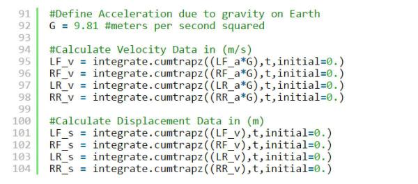
Figure 12: Python Velocity and Displacement Algorithm
Step 5: Plot acceleration, velocity, and displacement.
The source code pictured in Figure 13 generates a set of three graphs showing acceleration, velocity, and displacement with respect to time for the four corners of our test plate. A more in-depth description of 2-D plotting with Python and Matplotlib was discussed in Part 1 of this article series.
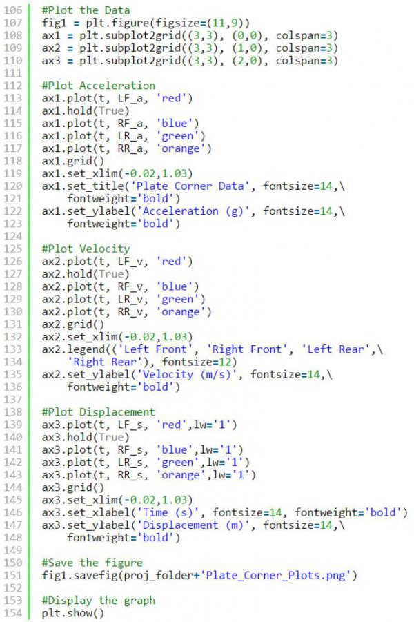
Figure 13: Python Data Plotting Algorithm
Step 6: Set up the 3D animation environment.
Now that we have the displacement data we need, we can start to set up the 3-D environment that we will use for our animation. This is where the VPython 3-D graphics module called “visual” comes into play. VPython makes it easy to create navigable 3-D displays and animations. First, we define the 3-D scene with the source code pictured in Figure 14, lines 157–162.

Figure 14: Defining the 3‐D Scene
In the source code pictured in Figure 15, we define (on line 165) a 3-D object called “ground,” which takes the form of a semi-transparent box. We then define the length (L) and width (W) dimensions of our test plate on lines 169–170. On lines 173–177, color-coded spheres are created to represent the corner points of our test plate. On lines 180–182, a multi-segmented curve is added to define the plate edges. Finally, we add labels on lines 185–196 to help identify each of the corners of the test plate.
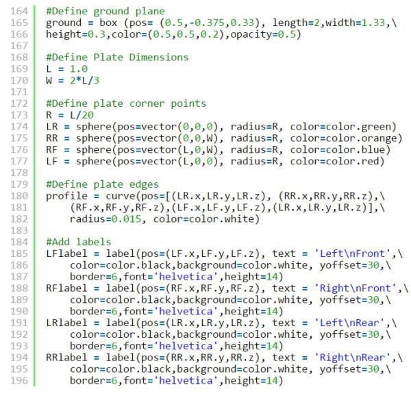
Figure 15: Defining 3‐D Objects
If we were to stop here, the program would generate the navigable 3-D display illustrated in Figure 16. To make objects move within the display, we need to add more code and use the displacement data we obtained earlier to create an animation sequence.
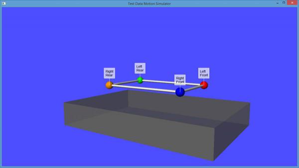
Figure 16: 3‐D Objects at Start of Animation Sequence
Step 7: Create a 3-D animation sequence
The source code pictured in Figure 17 is used to set up the animation sequence by creating an initial “pre-shot” time delay or countdown on line 199 so that when the display is first rendered, no motion is taking place until the time delay is completed. Before the animation loop begins on line 206, the initial value for the time variable (t1) is set to the first value in the time data array on line 202 and the loop continuation variable is set to true on line 205. The animation loop contains a rate() statement to limit the number of loop iterations/second on line 208. In this case, we use the sample rate (sr) as the limiting factor.
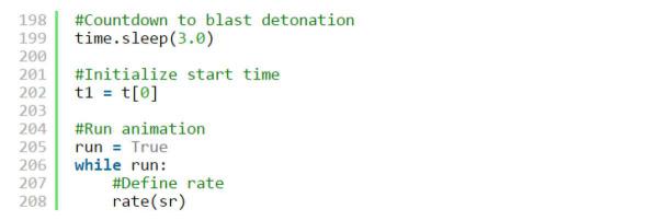
Figure 17: Animation Source Code
In lines 211–214 of the source code pictured in Figure 18, the test plate corner marker vertical position (y) values are updated based on the previously calculated vertical displacement array values corresponding to the current time (t1) value. Maintaining constant plate length and width dimensions and using Pythagoras’s theorem allow for the updating of the horizontal (x) and lateral (z) corner positions on lines 215–218. The plate edges are then updated to correspond to the new corner positions on lines 221–223, and the label positions are updated on lines 226–229. Advancing of the time step on line 232 prepares the way for the next pass through the animation loop. Finally, lines 235–236 terminate the animation loop when t1 reaches a value greater than the last value in the time array.
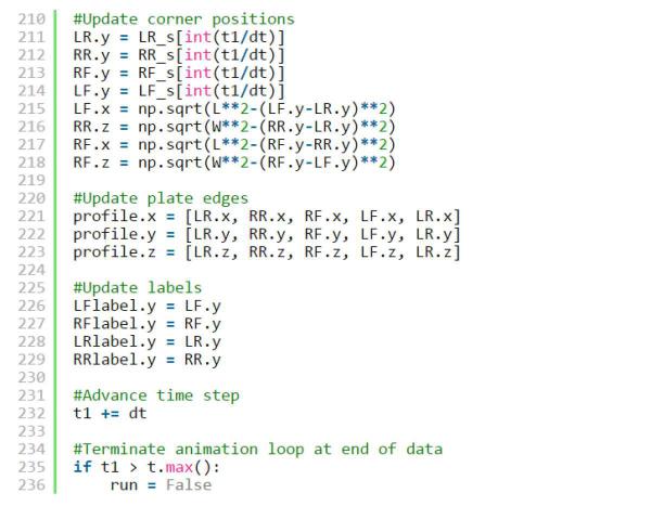
Figure 18: Creating the Animation Sequence
The VPython navigable 3-D display window remains open for user interaction after the plate animation has completed with the plate objects in their final positions at the end of the event, as illustrated in Figure 19.
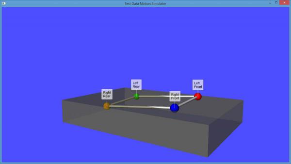
Figure 19: 3‐D Objects at End of Animation Sequence
Notice the plate appears to be partially buried in the ground object. This is a plausible situation in a blast event due to the crater created by the blast. That said, a word of caution is probably appropriate here with regard to data quality. Depending on several factors, including the placement and type of accelerometers used, the test data one has on hand may not be suitable for calculation of velocity and displacement and would therefore be unusable for animation purposes.
In conclusion, it has been shown here that if one has a suitable set of test data, creating 3-D animations using Python and VPython is not difficult and can be quite useful for visualizing test event motion. And with a little imagination and a proper application of math and physics, the animation possibilities are virtually limitless.