


INTRODUCTION
As defined in NAVAIR 00-25-403, Reliability-Centered Maintenance (RCM) is “an analytical process to determine appropriate failure management strategies, including Preventive Maintenance and other actions that are warranted to ensure safe operation and cost-wise readiness” [1]. Similarly, NASA defines the purpose of RCM as “a process that is used to determine the most effective approach to maintenance. It involves identifying actions that, when taken, will reduce the probability of failure and which are the most cost-effective” [2].
Over the years, RCM has been used to achieve significant cost savings on a variety of programs. For example, RCM performed on the F-15 environmental control, fuel, landing gear, flight control, and oxygen and canopy systems resulted in 538 recommended changes to the maintenance procedures with an expected savings of $21 million/ year (450,000 manhours) [3]. Likewise, since 1997, shipboard fleet maintenance manhours have been reduced by nearly 50% through the implementation of RCM principles [3].
The objective of an effective RCM program is not to eliminate failures but to reduce or mitigate the consequences of a failure when one occurs. The consequences of failure are usually assessed by their impact in the following four areas [4].
- Personnel and Equipment Safety
- Environmental Health/Compliance
- Operations (Availability)
- Economics
One of the defining characteristics of RCM is preventive maintenance (PM), which refers to actions performed periodically (or continuously) prior to functional failure to achieve the desired level of safety and reliability for an item. An effective RCM program strives to identify the PM necessary to ensure personnel safety, protect the equipment and environment, and ensure that the equipment will satisfy its operating requirements, and at a cost less than that of correcting the failure that the preventive task was trying to avoid.
PM tasks may be condition-directed (CD) or time-directed (TD). A CD-PM task is a periodic diagnostic test or inspection designed to detect a potential failure condition prior to functional failure. This detection is accomplished by comparing the existing material condition or performance of an item with established standards and taking further action accordingly. The objective of CD-PM is to maximize the useful life of each piece of equipment by allowing operation until a potential failure is detected. A TD-PM task is one that is performed to restore or replace an item before it reaches an age at which the probability of failure significantly increases. The restoration or replacement occurs regardless of the item’s actual material condition. TD-PM tasks may be appropriate when a failure mode does not exhibit characteristics that demonstrate a detectable reduction in failure resistance or the PM interval (the time between potential failure indication and actual failure) is not long enough to permit a CD task.
To determine the optimal time to schedule a TD-PM task, a maintenance planner must understand the time-dependent probability of failure of the targeted item relative to the expected life of the system. This article highlights how Weibull analysis can be used to analyze test or field-failure data to determine whether TD-PM is appropriate and, if so, determine the optimum replacement time. If warranted, Weibull analysis results can also be combined with cost data and reliability performance requirements to determine the optimum maintenance time.
RCM AND PM
RCM requires a disciplined approach to maintenance. Because resources (hardware, test equipment, personnel, time, funding, etc.) are limited, PM for all functional failure modes is simply not affordable and, at times, not even advisable. As a result, PM must be prioritized so that operational risks are reduced to an acceptable level and so that cost efficiency in the maintenance process is achieved. One method of prioritizing PM is summarized in Table 1.
| Failure Class | Class Description | PM Requirements |
| Critical Safety | Impacts operating safety where safety is related to loss of life and limb. | PM is required and must be able to reduce risk to an acceptable level. Otherwise, item must be redesigned. If redesign is not possible, identified risk must be expressly accepted. |
| Operating Capability | Failure that has a direct and adverse effect on operational capability (mission). | PM is desired if it is effective in reducing probability or operational consequences to an acceptable level. |
| Other Regular Functions | Failure that does not affect safety or mission capability. Typically these failures impact support functions. | PM is desired if it is cost-effective in reducing corrective maintenance. |
| Hidden or Infrequent Functions | Failures that impact functions that are not observable by operators during normal operation. They are characterized by an item for which there is no immediate indication of malfunction or failure. | PM is required to reduce the risk of multiple failures or function unavailability to an acceptable level. |
The applicability of TD-PM is predicated on three fundamental assumptions: (1) the probability of failure of a new (or restored) item is less than that of the item currently installed; (2) the PM will reduce the probability of occurrence, unavailability or operational consequences to an acceptable level; and (3) the cost of performing PM will be less than the cost of correcting the failure after it occurs. PM will be ineffective for failures that are random in nature because a new item will be just as likely to fail as an in-service one. Even worse, PM would result in reliability degradation for failures that exhibit “infant mortality,” as a new item will be more likely to fail than an in-service one.
For PM to be desired, the probability of failure of a new item should be less than that of the original item. For example, if an item experiences an increased failure rate over time, but the degradation is so slow compared to the equipment operating life as to be insignificant, then PM would likely not be cost-effective. Likewise, if the risk or probability of failure is at an acceptable level, but the costs of PM and corrective maintenance (CM) are similar, then the lack of potential significant cost savings may result in a decision not to pursue PM. Ultimately, the decision to implement PM rests on the following:
- Reduced Safety Risk
- Reduce Impact on Operational Capability
- Economics.
To assess the effectiveness of PM, a full understanding of the pertinent functional failure modes, failure causes, consequences and probability of failure prior to and after maintenance and the cost of preventive vs. corrective maintenance is necessary to ensure that limited resources are used efficiently.
WEIBULL ANALYSIS APPROACH
Weibull analysis can be used to guide many of the decisions related to PM. One of the results of a Weibull analysis is an estimate of the percentage of a population that will have failed prior to a given period of time. This information is crucial for determining when an item should proactively be restored or replaced. It can also be used to determine the optimal warranty period that minimizes customer dissatisfaction while preventing excessive replacement costs.
Four equations that describe the Weibull distribution and are necessary to determine the applicability of PM are shown in Table 2 [6].
| Description | Equation |
| Hazard Rate: | |
| Probabiliby Density Function (PDF): | |
| Cumulative Density Function (CDF): | |
| Reliability Function: |
Beta (β) is the Weibull shape parameter. It determines the shape of the Weibull distribution that best fits the data. It is the slope of the best fit line on the Weibull plot. Eta (η) is the Weibull scale parameter. Known also as an item’s characteristic life, it is defined as the time at which 63.2% of the population has failed. The variable “t” is the time at which the Weibull equations are to be evaluated.
The hazard rate, also known as the instantaneous failure rate, describes how the surviving members of a part population are failing at a given time. If the shape parameter (β) is less than 1, then the hazard rate is decreasing with time, and the item is said to be experiencing infant mortality. In this case, PM would not be advisable because a new component would statistically be more likely to fail than one currently in service. If the shape parameter equals 1, then the hazard rate is constant and is equal to the reciprocal of the characteristic life. PM would not be advisable in this case because a new item would be just as likely to fail as one currently in service, given that it has survived up to that point. Because failures are randomly occurring, PM would not do anything to improve mission success but would negatively impact availability and total maintenance cost. Consider, for example, the data provided in the Weibull plot shown in Figure 1.
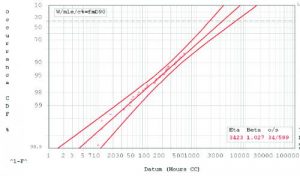
Figure 1: Weibull Data for a (Nearly) Exponential Case.
In this case, the shape parameter is 1.027, indicating an exponential (or nearly exponential) distribution, with a resulting constant (or nearly constant) failure rate. The characteristic life is 3,423 hr. Using the following CM and PM data (MTTRcorr = 5 hr; MTTRprev = 2 hr; CM cost = $30,000; PM cost = $5,000), the impact per unit of varying PM intervals on probability of failure, achieved availability, and total maintenance cost over a 4,000-hr operating period is shown in Table 3.
| PM Interval | Probability of Failure @ 4,000 hr | CM Actions | PM Actions | Achieved Availability | CM Cost | PM Cost | Total Maintenance Cost per Unit |
| None | 0.691 | 1 | 0 | 0.999 | $30,000 | $0 | $30,000 |
| 2,000 | 0.684 | 1 | 2 | 0.999 | $30,000 | $10,000 | $40,000 |
| 1,000 | 0.677 | 1 | 4 | 0.997 | $30,000 | $20,000 | $50,000 |
| 500 | 0.670 | 1 | 8 | 0.995 | $30,000 | $40,000 | $70,000 |
| 400 | 0.668 | 1 | 10 | 0.994 | $30,000 | $50,000 | $80,000 |
| 200 | 0.661 | 1 | 20 | 0.989 | $30,000 | $100,000 | $130,000 |
| 100 | 0.654 | 1 | 40 | 0.979 | $30,000 | $200,000 | $230,000 |
| 50 | 0.647 | 1 | 80 | 0.960 | $30,000 | $400,000 | $430,000 |
As Table 3 indicates, although the probability of failure slightly decreases (69.1% reduced to 64.7%), the achieved availability is negatively affected by more frequent PM (99.9% reduced to 96%). Therefore, although the unit may fail slightly less often with more frequent PM, it will spend a greater percentage of its time out of service. Additionally, the total maintenance cost increases significantly with increasing frequency of PM, even though CM is more costly on a per unit basis. It is clear from this example that PM would not be recommended and the units should be allowed to operate to failure. If the probability of failure shown here is a safety or mission risk, redesign would be the preferred option because improvement in this area would not be possible through PM.
If the shape parameter is significantly greater than 1, then the equipment is likely experiencing wear-out. Thus, a new or restored item would be less likely to fail than one currently in service. Thus, PM may be beneficial in reducing the probability of failure and/ or reducing maintenance costs. Safety and mission specifications, the relative cost of PM and CM, the steepness of the Weibull curve, and the magnitude of the characteristic life relative to the equipment life expectancy would be the factors that dictate whether (and with what frequency) PM should be applied. Weibull plots with steep slopes tend to have a more clearly defined region, where the increase in the probability of failure accelerates. If the equipment will be retired prior to this point, then PM may not be necessary, as failure would be highly unlikely. Alternatively, if the equipment will still be in service at this time, then PM may be scheduled to ensure that safety and mission specifications are satisfied. If the equipment is not safety- or mission-critical, economic failures may drive the decision. The more gradual the slope of the Weibull curve, the more difficult it is to determine the course of action; but the same principles apply.
Consider the data provided in the Weibull plot shown in Figure 2. In this case, the shape parameter is 1.62, indicating that wear-out is occurring with an increasing failure rate. The characteristic life is 1,728 hours. Using the same CM and PM data as in the previous example, the impact per unit of varying PM intervals on probability of failure, achieved availability, and total maintenance cost over a 4,000-hr operating period is shown in Table 4.
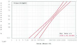
Figure 2: Weibull Data for a Wear-Out Case.
| PM Interval | Probability of Failure @ 4,000 hr | CM Actions | PM Actions | Achieved Availability | CM Cost | PM Cost | Total Maintenance Cost per Unit |
| None | 0.890 | 4 | 0 | 0.997 | $120,000 | $0 | $120,000 |
| 2,000 | 0.921 | 3 | 2 | 0.998 | $90,000 | $10,000 | $100,000 |
| 1,000 | 0.808 | 2 | 4 | 0.997 | $60,000 | $20,000 | $80,000 |
| 500 | 0.658 | 1 | 8 | 0.995 | $30,000 | $40,000 | $70,000 |
| 400 | 0.607 | 1 | 10 | 0.994 | $30,000 | $50,000 | $80,000 |
| 200 | 0.456 | 1 | 20 | 0.989 | $30,000 | $100,000 | $130,000 |
| 100 | 0.327 | 0 | 40 | 0.980 | $0 | $200,000 | $200,000 |
| 50 | 0.227 | 0 | 80 | 0.962 | $0 | $400,000 | $400,000 |
As Table 4 indicates, the probability of failure is significantly impacted by PM (98% at 4,000 hr when operated to failure vs. 22.7% at 4,000 hr with PM being performed every 50 hr). On the other hand, the achieved availability is negatively affected by more frequent PM (99.7% reduced to 96.2%). Therefore, although the unit is likely to fail significantly less often with more frequent PM, it will spend a greater percentage of its time out of service. If minimizing the probability of failure is the overriding concern, then an increased frequency of PM is recommended.
For example, if the item is required to have a probability of failure of less than 35% at 4,000 hr, then PM must be performed at least every 100 hr. If maximizing availability is the goal, then PM performed at intervals of 500 hr or greater would be recommended, with maximum availability being achieved at 2,000-hr intervals. If maintenance cost is to be minimized, 500-hr interval would be recommended.
Finally, the expected length of service should also be considered, as it will affect the conclusions. Table 5 shows the analysis results from the same data set as used in the previous example, except that the length of service is 600 hr.
| PM Interval | Probability of Failure @ 600 hr | CM Actions | PM Actions | Achieved Availability | CM Cost | PM Cost | Total Maintenance Cost per Unit |
| None | 0.165 | 0 | 0 | 0.997 | $0 | $0 | $0 |
| 300 | 0.111 | 0 | 2 | 0.993 | $0 | $10,000 | $10,000 |
| 200 | 0.087 | 0 | 3 | 0.990 | $0 | $15,000 | $15,000 |
| 100 | 0.058 | 0 | 6 | 0.980 | $0 | $30,000 | $30,000 |
| 50 | 0.038 | 0 | 12 | 0.962 | $0 | $60,000 | $60,000 |
As Table 5 suggests, as long as the probability of failure and availability requirements are satisfied, no PM would be recommended.
SUMMARY
The discussion and examples presented in this article show how Weibull analysis can be used to guide TD-PM strategy. Understanding the underlying failure distribution of an item is critical in determining whether or not PM is appropriate, and at what interval. Equally important is the understanding of PM and CM times, preventive and corrective replacement costs, and equipment design life. Finally, a clear understanding of safety and mission reliability requirements is also necessary for an optimal PM program.
References:
- NAVAIR 00-25-403. “Guidelines for the Naval Aviation Reliability-Centered Maintenance Process.” Naval Air Systems Command, 01 July 2005.
- “Reliability Centered Maintenance Guide for Facilities and Collateral Equipment.” National Aeronautics and Space Administration, February 2000.
- “Reliability Centered Maintenance.” Office of the Under Secretary of Defense for Acquisition, Technology, and Logistics (OUSD(AT&L)). N.p., 17 Oct 2006. Web. 13 Nov 2014. <http://www.acq.osd.mil/log/mr/rcm/RCM_brochure.pdf>.
- Wisniewski, R. “Quanterion RELease Series: Reliability Centered Maintenance.” Quanterion Solutions Incorporated, 2013.
- S9081-AB-GIB-010. “Reliability-Centered Maintenance (RCM) Handbook.” Revision 1, Naval Sea Systems Command, 18 April 2007.
- Lein, P. “Quanterion RELease Series: Weibull