


INTRODUCTION
Improvised explosive devices (IEDs) have proven to be highly lethal tools frequently used in asymmetric warfare. This has been particularly true of explosively formed penetrator (EFP)-based IEDs. Many of these devices are either manufactured by foreign entities, in the manner in which “ordinary” production EFPs are produced, or they are crudely manufactured in a local setting. Regardless of the precise nature and location of their manufacture, however, they are often produced so imprecisely that proper formation of the EFP appears to have been an afterthought relative to simply inflicting damage against thinned vehicles and their occupants. The Combat Capabilities Development Command Armaments Center (CCDC AC) characterized the performance of a simple, improvised device found in a foreign theater. This article outlines the effort to characterize the penetration performance of three improvised, copper, 4-inch-diameter EFPs recovered from the field. High-rate continuum modeling was used to understand the limits of the penetration capability of these devices and the implications of the manner in which they were produced so that the threat they pose could be accurately assessed.
In the most recent campaigns conducted by the United States and its allies, EFPs have been used against friendly forces with a high degree of effectiveness [1–3]. Later in the war as standard military-grade devices became too difficult or dangerous to obtain, homemade explosives started entering the scene. Not only did the types of explosives used to drive IEDs change, but their nature changed as well. In Iraq, there was a rapid change from the initial use of buried military- grade ordnance to improvised explosively formed penetrators (EFPs). In 2004, EFPs made their initial entrance into the Iraqi theater [4–7]. Because of a variety of tactical benefits, EFPs were often chosen by insurgents against coalition vehicles.
The lethal effectiveness of EFP IEDs motivated a rapid and extensive change in coalition tactics, techniques, and procedures, including the use of electronic and physical countermeasures like Warlock and Rhino, among others [8–10]. In as early as 2003, high-mobility, multi-wheeled vehicle (HMMWV) armor levels increased. Later in 2007, mine-resistant, ambush-protected vehicles like the Cougars and Buffalo began to see initial operational use [11, 12]. As a result of dwindling stockpiles of military-grade munitions and explosives, insurgents resorted to using improvised EFPs. The liner shown in Figure 1 is an improvised, 4-inch-diameter, copper EFP. The ultimate goal of this effort was to understand and characterize the performance of this device.
CHARACTERIZATION MODELING
In order to characterize the potential performance of this EFP, a computer model first had to be developed from previously-acquired samples. One of these liners can be seen in Figure 1. From visual examination of this liner, it appears to have been pressed from low-purity copper, measuring roughly 3 mm thick. The liner depth measured 0.85 inches, a value that is only approximately 22% of the total liner diameter and is indicative of a lack of familiarity with traditional EFP designs. By our standards, this liner was crudely formed—composed of at least two different radii joined by a discontinuity. Subsequently, its performance was anticipated to be low because prior experimental observation of devices like these showed that the penetrator tended to break up only a short distance away from its original positions [13].

Figure 1: Improvised Liner (Source: CCDC AC).
It appears as if minimal machining was conducted to clean up the outer circumference. An immediately apparent artifact of its manufacturing technique (observable in Figure 1) was the existence of a flat on both surfaces. This flat resulted in a noticeable discontinuity where it met the radii on both sides of the liner surface.
Although no body was recovered, it was assumed that the device was designed to be assembled inside a plastic housing. The length-to-diameter ratio of this body was kept to 1 for convenience. Composition C-4 was used as the driving explosive because of its availability and ease of use. From prior experience, a device of this caliber and precision was believed to be accurate out to maximum range of approximately 50 ft, with a “modest” penetration potential of only about 1.5 inches of steel. This was more than enough to penetrate thin-skinned vehicles.
Before proceeding with experimental characterization, CCDC engineers created a baseline solid model using PTC Creo from somewhat crude measurements taken using a Vernier caliper (Figure 2).

Figure 2: Improvised EFP Solid Model (Source: CCDC AC).
To generate this model, the following simplifying assumptions had to be made: the liner had a constant thickness of 3 mm, and the curvature of the liner was composed of two different curves that met at the surface discontinuity previously discussed. Although little was known about how this device was loaded, with what explosive, and whether or not it was boosted among other variables, a simplified set of simulations was generated.
All simulations were conducted using Lawrence Livermore National Laboratories code ALE3D (Table 1). An example of the baseline simulation at time 0 can be seen in Figure 3. An early time snapshot shows it folding rearward and breaking in Figure 4. A Johnson-Cook constitutive model was used for the copper liner in all simulations. The body was modeled using a Mie-Grüneisen equation of state, and the target was modeled using an internal material model. Approximately 10 elements per centimeter were used for all simulations.
Table 1: Baseline Simulations

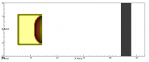
Figure 3: Baseline Penetration Model (Source: CCDC AC).

Figure 4: Baseline Model at 50 and 90 μs (Source: CCDC AC).
After only about 60 µs, the penetrator tip separated from the rest of the body. This was not surprising given the visible discontinuity in the liner. Predictably, the velocity of the broken tip was much higher at around 2.2 km/s, while the remaining penetrator travelled at only around 1.5 km/s. Because the penetrator was both hollow and broken, it was highly likely that the penetration performance would be low. The computational results are tabulated in Table 2.
Table 2: Baseline Performance

LINER MEASUREMENT AND TESTING
Subsequent to initial modeling, a coordinate measuring machine (CMM) was used to verify the degree of agreement with the previous baseline and understand liner consistency and symmetry. It is important to point out that because these liners were not created from a solid model, no solid modeling profile data were obtainable and, therefore, the data normally used for comparison did not exist. Perpendicular diameters were measured on both surfaces and broken down into two parts regarding their coordinate system. They were labeled as Zplus, Zminus, Xplus, and Xminus lines, with the positive y direction normal to the air side of the liner. Two circumferential measurements were also taken at different radii to assess profile consistency. An outline of a simplified set of this data can be seen in Figure 5.

Figure 5: CMM Profile Measurements (Source: CCDC AC).
All of the radial measurement data were then plotted to highlight any asymmetries, as shown in Figure 6. Although each liner had an average diameter measuring a little over 4 inches, CMM data were generally only recorded out to a little under that diameter, as the process used to part the liner near the outer diameter left a rough, beveled outer edge. As a result, including any data past the outer circumference would have appeared to decrease the liner’s geometric fidelity, so it was disregarded.

Figure 6: Liner 1 Profile Measurements (Source: CCDC AC).
Whatever manufacturing technique was used, it resulted in reasonably consistent results near the liner’s apex, with a far greater degree of variability near the outermost diameter. Tabulated measurement results are listed in Table 3.
Table 3: Part 1 Liner Thickness Variations

These values were calculated by subtracting all of the values taken in the y direction on the concave side of the liner from those on the convex side. They were not measured normal to either the convex or concave surface but were simply differences in the measured y values taken along the various radial lines at different y points. If we disregard this somewhat crude numerical technique, we note several important features. For example, even though each line seems to indicate that liner measurement varies less than 0.0005 inches at the apex, there is a consistent but slight thinning of the material as one proceeds outward along the radial direction. What results is a variable liner profile that is thickest at the apex and outer diameter, with a thinner portion between the two. This was almost certainly an artifact of the manufacturing technique.
Secondly, it is apparent that these liners were not perfectly symmetric. From one quadrant to the next, maximum thicknesses were measured at different axial locations. In the second quadrant, a maximum liner thickness was measured at over 0.5 inches from the origin of the axis; however, this value was closer to 0.9 inches in the first quadrant. This is a tremendous difference that can only contribute to degraded performance. When these variations are coupled with others in high-explosive type, density, and metallurgical quality, penetration and accuracy are likely to suffer appreciably. We were unable to test accuracy over distance, however, because of the short range of our test facility.
When these variations are coupled with others in high-explosive type, density, and metallurgical quality, penetration and accuracy are likely to suffer appreciably.
Further variations can be seen by examining the data measured at the two radial distances shown in Figure 5. When we look at the data along these circles and compare them to ideal circles of identical radii, we see that the liner thickness varies from over 0.001 inches to almost 0.005 inches. This too is an appreciable difference that would not ordinarily be acceptable in an environment necessary to produce high-performance liners.
The CMM data we collected were limited because of the speed with which the results of this evaluation were required. Even if more data had been gathered, it would have been prohibitively difficult to use this information to generate a higher-fidelity, solid model. With the tools we had at the time, we would have had to make assumptions about how the liner transitioned from one quadrant to the next. If we only measured two radial lines along a single diameter, we might assume that if the thicknesses were different, it changed linearly from one quadrant to the next. This would have been without any physical basis but would have made the problem numerically more tractable. As a result, the modeling used at least a subset of the four-point quadrant data shown in Figure 6 as this was an approximation that allowed a reasonable degree of error while minimizing other errors.
The first test we conducted used 150-kV x-ray heads fired at 190 and 350 μs of delay from initiation time. The components’ mass is tabulated in Table 4. Late times were chosen to accommodate the test configuration and the need to protect the x-ray films. We could not obtain early formation times prior to 130 μs, making any comparison to the early time formation predicted via modeling impossible. The test setup is shown in Figure 7, while the model and x-rays can be seen in Figure 8.
Table 4: Shots 1 and 2 Mass


Figure 7: Test Setup (Source: CCDC AC).

Figure 8: Late Time X-rays Taken at 190 and 350 μs (Top and Middle) Compared to the Model at 350 μs (Bottom) (Source: CCDC AC).
Unfortunately, the segment of shot 1 film containing the fiducial rod was damaged. As a result, measuring velocity had to be conducted differently from the manner in which it would ordinarily be obtained. Instead, the distance the particles traveled was measured from the film. This distance, combined with knowing the times at which x-rays were fired, provided a somewhat crude mechanism to measure tip velocity (of the broken region) for shot 1 of 2.4 km/s. The calculated velocity was 2.3 km/s. The first large “particle” velocities measured roughly 1.9 and 1.85 km/s for shots 1 and 2, respectively. For shot 2, the lead particle had already exited the film area, so no calculation of velocity was possible. Penetration for both shots was in line with the higher end of the predicted value of 1.5 to 1.75 inches. Both target plates exhibited peripheral damage indicative of the fragmentation shown on the x-ray films (Figure 9).

Figure 9: Steel witness plate penetration for Shot 1 (Left) and Shot 2 (Right) (Source: CCDC AC).
Experiments and modeling resulted in general agreement for predicted velocity and penetration depth, with appreciable differences with the breakup. The copper was modeled using the well-known Johnson-Cook constitutive equation with failure. (This type of model is usually applied to high-quality, high-purity copper.) The pedigree of the tested liner was completely unknown but believed to be a common, industrially-obtainable grade. Based on the x-rays taken during flight, the liner failed in a manner that could only be described as brittle. Whether the copper comes from sheet or bar stock, is forged from ingot, or is pure makes a tremendous difference in performance. In our estimation, these liners were unlikely to have come from high-quality copper used in traditional designs for which the Johnson-Cook model is most typically applied.
The initial metallurgical condition was also unknown, as was the heat treatment and level of work that were put into the material. Judging by the precision of the liner, however, it was highly likely that no additional heat treatment occurred. As a result, the ductility of the tested liner was likely far lower than modeled. Relative to other x-rayed EFPs, it appears as if the failure exhibited by this liner was brittle in nature. We believe that the type of copper used in these liners was electrolytic tough pitch (ETP). This type of copper is not commonly used in modern, high-performance EFPs because of its deleterious effect on performance.
CONCLUSIONS
The baseline performance of an improvised, copper EFP was modeled using ALE3D. Agreement between the prediction and experimental data varied, with only modest agreement for early time formation. Predicted penetration performance agreed much better with modeling. Although there are likely a number of causes for early time formation differences, our primary hypothesis is that the material model we used to model the copper was different from the actual copper used in the item.
In the absence of compositional analysis, attributable to only having a low number of test articles, and because the constitutive and failure models depend upon such a composition, it is impossible to determine if this was the precise cause of the differences. There were, however, several other potential reasons for the observed variation between modeling and experiment. These include, but are not limited to, the simplified liner symmetry and profile necessary to begin modeling. From testing, we can safely conclude that although there were numerous and appreciable imperfections in this liner, it is highly probable that its performance against thin-skinned vehicles like trucks or HMMWVs would be sufficient, albeit inconsistent, depending on the quality of the explosive loading, type of housing, and precision of assembly, among other factors.
Although there were numerous and appreciable imperfections in this liner, it is highly probable that its performance against thin-skinned vehicles like trucks or HMMWVs would be sufficient.
- Welch, A. “Iraq – The Evolution of the IED.” CBRNe World, http://www.cbrneworld.com/_uploads/download_ magazines/08_autumn_IRAQ_EVOLUTION_OF_THE_IED.pdf, 2008.
- Fahim, K., and L. Sly. “Lethal Roadside Bomb That Killed Scores of U.S. Troops Reappears in Iraq.” The Washington Post, October 2017.
- Eisenstadt, M., M. Knights, and A. Ali. “Iran’s Influence in Iraq Countering Tehran’s Whole-of-Government Approach.” Policy focus #111, https://www.washingtoninstitute.org/uploads/Documents/pubs/PolicyFocus111.pdf, April 2011.
- Conroy, S. “U.S. Sees New Weapon in Iraq: Iranian EFPs.” CBS News, https://www.washingtoninstitute.org/uploads/Documents/pubs/PolicyFocus11…, 11 February 2007.
- Hambling, D. “EFP In Iraq: Deadly Numbers.” https://www.wired.com/2007/08/superbombs-the/, 22 August 2007.
- Crown. “The Report of the Iraq Inquiry. Report of a Committee of Privy Counsellors.” United Kingdom House of Commons report, vol. XI, http://www.gov.uk/government/publications, 2016.
- Morgan, D. “Iraq Sunni Insurgents Turn to Armor-Piercing Bombs.” Reuters, 7 February 2008.
- Russ, D. “The Silent War.” https://civilianmilitary-intelligencegroup.com/8264/the-silent-war-bombe…, 10 July 2011.
- Joint Improvised Explosive Device Defeat Organization (JIEDO). “Attack the Network – Defeat the Device – Train the Force.” Annual report, 2008.
- JIEDO. “DOD’s Fight Against IEDs Today and Tomorrow.” U.S. House of Representatives Committee on Armed Services Subcommittee on Oversight and Investigations, November 2008.
- Wasrner, F. “Army Stepping up Its Humvee Orders for Troops in Iraq.” https://www.nytimes.com/2003/12/25/business/army-stepping-up-its-humvee-…, 25 December 2003.
- Blakeman, S. T., A. R. Gibbs, and J. Jeyasingam. “Study of the Mine Resistant Ambush Protected (MRAP) Vehicle Program as a Model for Rapid Defense Acquisitions.” MBA professional report, Naval Postgraduate School, Monterey, CA, 2008.
- Bender, D., and J. Carleone. “Explosively Formed Projectiles.” Tactical Missile Warheads. Boulder: American Institute of Astronautics and Aeronautics, pp. 367–386, 1993.